8. Delayed Mode Quality Control

8.1. Time synchronization

As many glider users are familiar with, it is essential to sync the time between the glider and their sensors. With the HydroC CO₂ this is carried out when the sensor is turned on with a clock-sync with gps. The internal clock in the HydroC is stable, so this only needs to happen at the beginning of the mission or in the lab before deployment.

8.2. Geometrical alignment

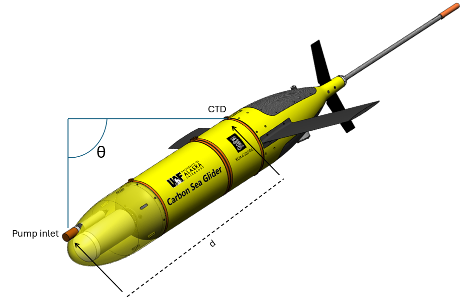
Since the HydroC CO₂ is integrated into the nosecone of the seaglider, forward of the standard CTD location near the aft hatch, geometric alignment is necessary to determine the exact location where a pCO₂ measurement was recorded. Because the pCO₂ signal needs to be corrected for response time, it is easier to find the pressure at the location of the pCO₂ measurement (e.g. see [Woo and Gourcuff, 2023]) rather than finding the time offset and further convoluting the response time correction. This can be accomplished using geometry (8.1).

(8.1)\[P_{Hydroc} = P_{CTD} - sin(θ)*d \]

Where P_HydroC is the pressure associated with the pCO₂ measurement, P_CTD is the pressure associated with the glider CTD measurement, θ is the glider pitch, and d is the distance between the sensors.

Fig. 8.1 Seaglider orientation during a dive showing the pressure at the location of the pCO₂ measurements (pump inlet), CTD location, and the distance between the two (d), as well as the pitch of the glider (θ).

8.3. Sensor response time correction

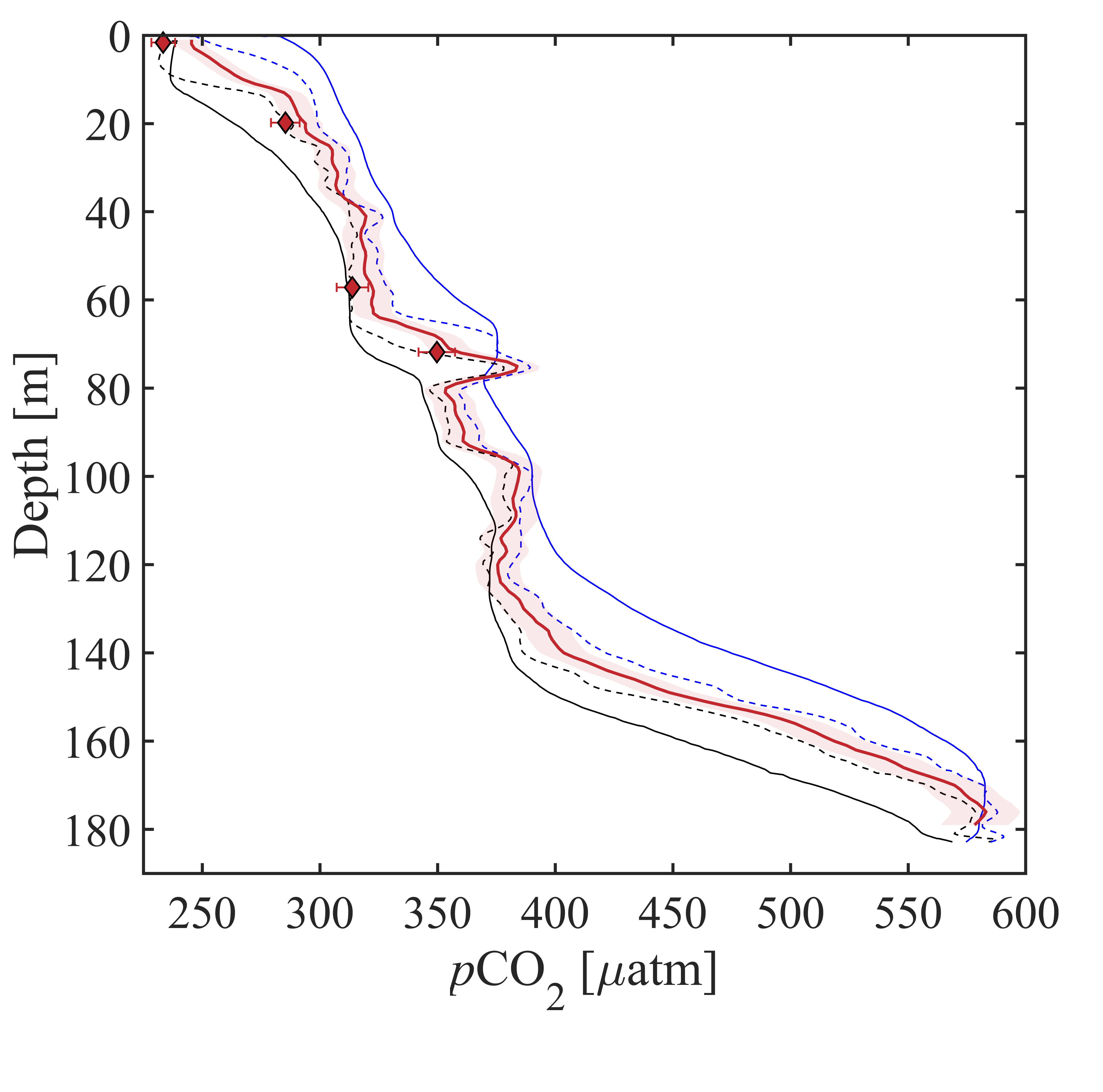
For equilibrium-based (EB) sensors, the sensor response time (RT) is directly governed by how fast the analyte can diffuse through the membrane. The ability to determine the in situ response time (τ₆₃ of the HydroC, which took into account membrane characteristics and the rate of water exchange over the membrane, i.e. pump characteristics) of the sensor makes correction for hysteresis through data post processing possible (Figure 8.1). Although the RTC method of [Miloshevich et al., 2004] has been previously used for HydroC CO2 correction from a profiling float [Fiedler et al., 2013] and is very simple to implement, the [Dølven et al., 2022] RTC method produced more realistic profiles. Additionally, [Dølven et al., 2022] developed their algorithm with equilibrium-based sensors in mind and was proven with a sensor with a long response time (HydroC CH4 𝝉63 ≅ 23 minutes) and provides an explicit uncertainty estimate of the response-time-corrected signal.

The [Dølven et al., 2022] RTC solution is based on the framework of statistical inverse problems and linear regression and assumes the relationship between observed quantity, ua(t), and measured quantity, um(t) is governed by the growth-law equation (eq 1 [Dølven et al., 2022]). Uses weighted linear least-squares estimator, the growth-law equation as measurement model, and a sparsity regularized solution.

Response time for the HydroC CO2T sensors are determined during calibration at -4H-JENA and are necessary for response time correction (RTC). Field verification of the response time is recommended to ensure the highest quality post-processed data product because τ₆₃ can be affected by the speed of water exchange across the membrane (e.g. pump speed, tube length, etc.), see Section 4.2.2.

Before RTC is applied, HydroC CO₂ data may need to be smoothed to avoid/limit erroneous spikes in the RTC signal. For our project, smoothing was applied using a quadratic regression (MATLAB’s smoothdata.m function with the loess method) over a 2-minute window to maintain the original 2 second resolution of the pCO₂ data.

Fig. 8.2 CO₂ Seaglider data from a sea trial mission in spring 2022 in Resurrection Bay, Seward, Alaska. Depth profile of pCO₂ in μatm showing the original resolution smoothed pCO₂ used in the RT correction (downcast = solid black, upcast = solid blue), RTC pCO₂ following [Dølven et al., 2022] (dashed black line = downcast, dashed blue line = upcast), and 1-meter binned RTC profile (thick red line) with red shading showing the relative uncertainty of 2.5 %. Discrete pCO₂^disc shown as red diamonds with horizontal red error bars showing combined standard uncertainty [Orr et al., 2018]. Figure from [Hauri et al., 2024].